Warning Still under development may not be accurate!

Tutorial 3 - Calculating the Tunneling Constant

Calculating the Tunneling Constant

Transfer integrals are an important of the charge transport rate equations. The two most common rate equations are the Miller and Abrahams Rate Equation and the semiclassical Marcus rate equation.

\[k_{ij} = \nu_0 e^{-2 \alpha r_{ij}} e^{- \frac{|\varepsilon_j - \varepsilon_i| - (\varepsilon_j - \varepsilon_i)}{k_B T}}\]

Here, \(\nu_0\) represents the attempt to hop frequency, \(\alpha\) sometimes written with a \(\gamma\) represents the tunneling constant or inverse localization length, \(r_{ij}\) is the distance between two sites, \(\varepsilon_i\) and \(\varepsilon_j\) are the energies of the sites, and \(k_B\) is the Boltzmann constant and \(T\) the temperature respectively.

\[k_{ij} = \frac{2 \pi}{\hbar} \frac{1}{4 \pi k_B T} |H_{AB}|^2 e^{-\frac{(\Delta G+\lambda)^2}{4 \pi \lambda }}\]

Here \(\hbar\) is Planck’s constant, \(\Delta G\) is Gibbs free energy, \(H_{AB}\) is the transfer integral sometimes it is denoted as \(J_{AB}\) and \(\lambda\) is the reorganization energy.

The Miller and Abrahams rate equation was developed heuristically but has been used quite successfully. On the other hand the Marcus rate equation developed by Rudolph Marcus (1992 Nobel Prize in chemistry) has been more rigorously derived from first principles. Regardless of whether you pick one or the other the transfer integral is a key component. If you want to enhance the analysis of your papers there are a few simple calculations that you can do. One of these is to calculate the tunneling constant. Often times people like to create an analytical expression to approximate the transfer integral as a function of distance this is explicitly written in the Miller and Abrahams equation above with the \(e^{-2 \alpha r_{ij}}\) term. The approximation can also be used with the Marcus rate equation when you consider that \(H_{AB}\) can essentially be written as:

\[|H_{AB}|^2 = |J_{AB}|^2 = J_0 e^{-2 \alpha r_{ij}}\]

Using this analytical expression then removes the need to calculate the transfer integral between every pair of molecules. Granted, this approximation is not always ideal especially when you have molecules that are asymmetrical in which case the orientation will play an important role.

For the purpose of this tutorial we will once again use an ethylene dimer to illustrate the calculations. Each calculation was run using the following Gaussian commands:

# b3lyp/6-31+g(d) nosymm geom=connectivity iop(3/33=1) punch=mo scf=tight

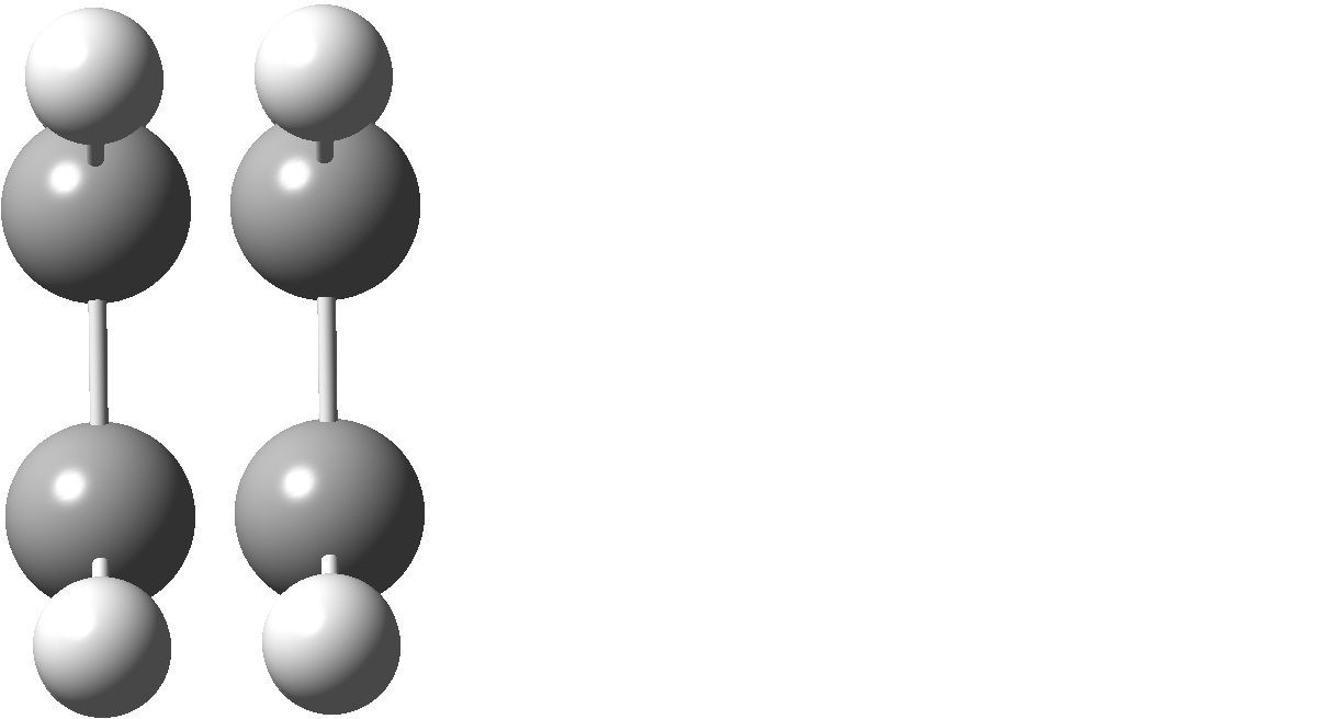
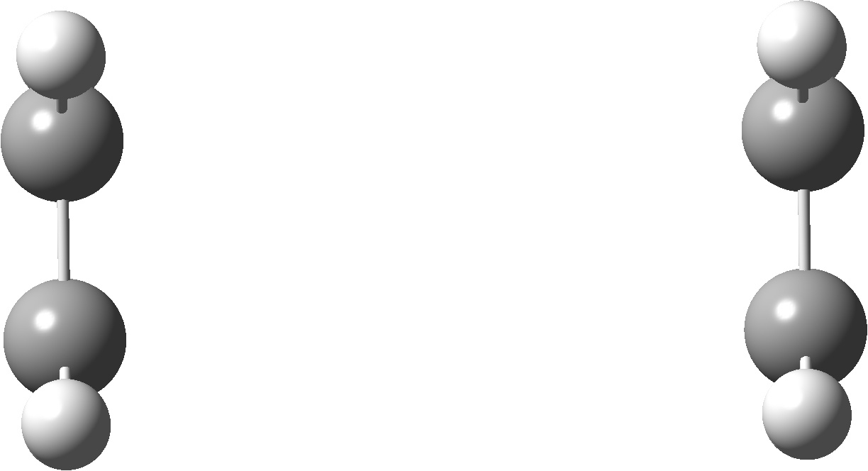
Several dimer calculations were run at different distances while keeping the molecules symmetrically orientated. As shown for ethylene molecules separated at a distance of 1 angstrom and 5 angstroms.

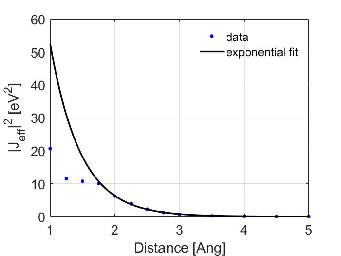
Using calc_J you can then calculate the effective transfer integrals. Now if we were interested in modeling charge transport for an electron we would look at the transfer integrals between the LUMO orbitals. However, organic semiconductors tend to be hole transport materials so I have instead calculated the transfer integrals between the HOMO values. By squaring them and fitting them to an exponential fit the tunneling constant can then be determined.

The fit shown above was made using matlabs cftools. Which calculated a best fit value for \(\alpha\) of 0.6441 and of \(J_0\) of 71.31. However, this is misleading as I have plotted in a linear scale. Look how poor the fit is when shown in the log scale.

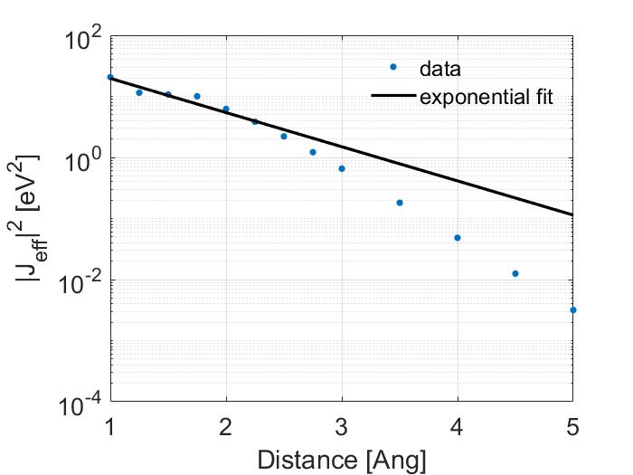
Note that the fit is poor for values less than 2 Ang. A better way to make a fit would be to exclude the values before 2 Ang so this is what I have done.

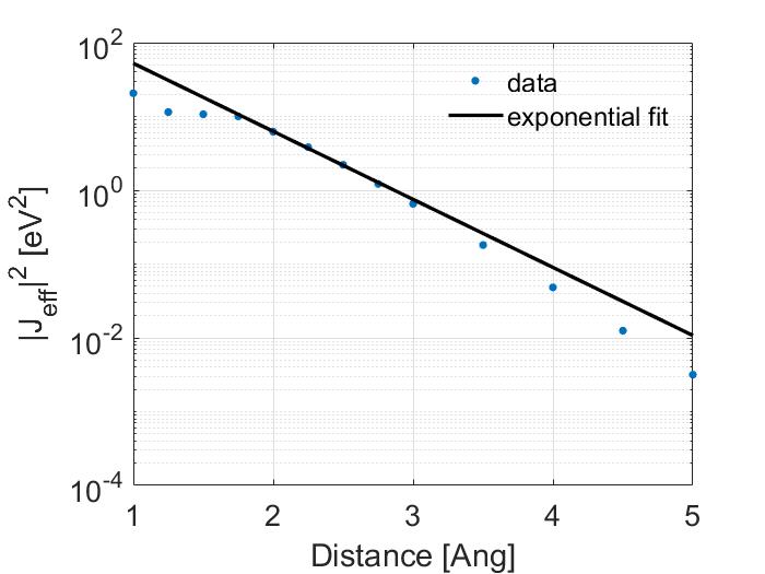
Here, I get much better values with \(\alpha\) of 1.0614 and of \(J_0\) of 438.1032. Note that at large distances the results start to diverge again, this is expected because I used a Gaussian basis set and is thus a limitation of using Gaussian functions to describe what in reality should be an exponential curve at large distances, if you wanted a better fit at larger distances I would recommend using a better basis set or a long range corrected functional. For your convenience I have also provided all the values that I calculated so you can compare your results with them.

Distance [Ang]	\(J_{eff}\) [eV]	\({J_{eff}}^2\) [eV^2]
1.00	4.5380	20.5937
1.25	3.3862	11.4666
1.50	3.2736	10.7163
1.75	3.1660	10.0236
2.00	2.4920	6.2100
2.25	1.9573	3.8309
2.50	1.4866	2.2099
2.75	1.1037	1.2182
3.00	0.8091	0.6547
3.50	0.4254	0.1809
4.00	0.2197	0.0483
4.50	0.1119	0.0125
5.00	0.0563	0.0032