Overview
In the previous simulation, I showed how to simulate a single charge moving along a 1d lattice. In this tutorial, we will expand on what we did previously but with several improvements by simulating a Time of Flight (ToF) experiment.
In this tutorial, we will model this experiment but with the improvements listed below.
- We will use a 3d lattice, with periodic boundaries on the y and z directions
- We will use the Marcus rate equation with the Gaussian Disorder model to generate our rates
- We will simulate several charges as opposed to just 1
- We will show how to calculate the current transient
ToF
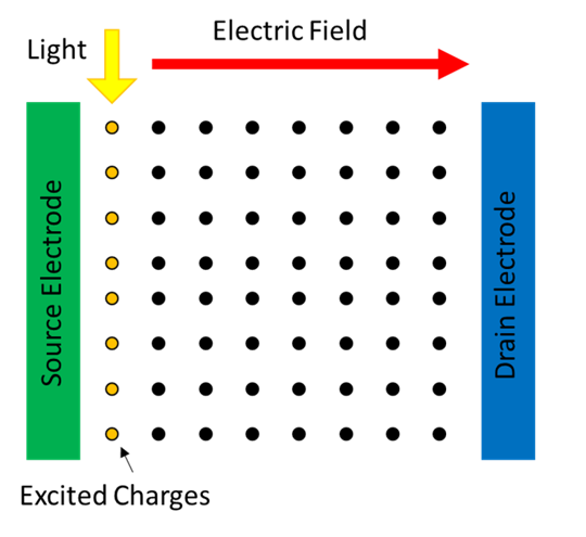
The goal of a ToF experiment is to calculate the carrier mobility, typically it is used with organic semiconductors. To setup a ToF experiment the semiconductor is sandwhiched between two electrodes. An electric field is applied across the electrodes to provide an energetic driver for any free carriers. Depending on the size of the band gap in the semiconductor there are likely to be few free carriers. To create some carriers light is used to optically excite charges on one side of the material. The electric field then facilitates movement of the charges to the opposing electrode generating a current.
Implementation of the ToF simulation is setup in 7 steps:
- Creating a Cubic Lattice
- Impart Material Qualities to the Lattice
- Calculate the Rates between Sites
- Exciting Charges
- Setting up the Coarse Graining System
- Creating a Queue
- The Main Loop
1. Creating a Cubic Lattice
Here we demonstrate a cubic lattice of sites. The MythiCaL library contains a convenience class specifically for this purpose which can easily be imported by including the right header file.
#include <mythical/charge_transport/cubic_lattice.hpp>
Once the header is imported, we can define out lattice. Below we have defined a lattice 200 by 80 by 80 sites where the spacing between each of the sites is a single nm. Our y and z boundaries have also been made periodic to avoid surface artifacts.
const int len = 200;
const int wid = 80;
const int hei = 80;
const double inter_site_dist = 1; // nm
const int total_num_sites = len * wid * hei;
myct::BoundarySetting x_b = myct::BoundarySetting::Fixed;
myct::BoundarySetting y_b = myct::BoundarySetting::Periodic;
myct::BoundarySetting z_b = myct::BoundarySetting::Periodic;
myct::Cubic lattice(len, wid, hei, inter_site_dist, x_b, y_b, z_b);
2. Impart Material Qualities to the Lattice
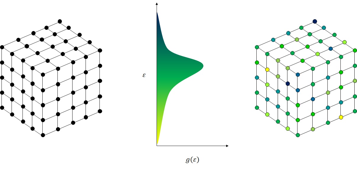
Having created a lattice, the next step involves making the lattice represent a material we are interested in. Each of our lattice points must have an energy associated with it. If we can accurately calculate what that energy should be then we are one step closer to correctly modeling the electrical properties of a real material.
A normal or Gaussian distribution is often used to represent the Density of States (DOS) of disordered semiconductors. We will assume this approximation holds here, but if one knew the shape of the DOS it could be used instead. We will also assume the carriers we are going to simulate are holes, so the DOS is assumed to be composed of the HOMO levels of molecules we are modeling.
By using a Gaussian distribution to model the DOS we can use the standard deviation of the Gaussian distribution as a metric to measure the disorder of our semiconductor. To give the reader some context of the size of this parameter, for AlQ3 values of 0.2 eV have been calculated [1], for α-NPT, spiro-DPVBi, TCTA [2] the standard deviation has been calculated to range from 0.10 – 0.156 eV and for several copolymers it has been found to range between 0.09 – 0.11 eV [3]. In general, a narrower DOS indicates less disorder which will lead to a higher carrier mobility.
One of the chief approximations of Gaussian Disorder Model, used by Bässler, is that the energies assigned to sites are uncorrelated. We will assume this approximation hold true, so we will randomly assign energies from the DOS to each of the sites without considering that sites in close proximity might be energetically similar. Thankfully the c++ standard library comes with a nice random number generator.
In the code snippet below, we know the total number of sites, so a vector instance equal to the number of sites is first initialized. Each site has a unique index thus by assigning an energy to each index of the vector (site_energies) all of the sites in the lattice are accounted for.
std::vector<double> generateSiteEnergies(const int & total_num_sites) {
  // Define our DOS as a normal distribution
  const double mean = -1.2; // eV
  const double std_deviation = 0.07; // eV
  std::normal_distribution<double> distribution(mean, std_deviation);

  // Randomly assign energies from our DOS to our lattice sites
  std::default_random_engine generator;
  std::vector<double> site_energies(total_num_sites);
  for(size_t index = 0; index < total_num_sites; ++index){
    site_energies.at(index) = distribution(generator);
  }
  return site_energies;
}
3. Calculate the Rates between Sites
The next step involves defining the hopping rates that govern charge movement between sites. We will calculate these rates using the semiclassical Marcus rate equation, though the Miller and Abrahams rate equation would also be appropriate.
\[k_ij = \frac{2\pi}{\hbar} \frac{1}{\sqrt{2 \pi \lambda k_B T}} |H_{AB}|^2 e^{ - \frac{(\lambda + \varepsilon_j - \varepsilon_i)^2}{4 \lambda k_B T} }\]- \(k_ij\) represents the hopping rate [1/s]
- \(\hbar\) is plank’s constant with a value of \(6.582119569 \times 10^{−16}\) [eV s]
- \(\lambda\) is the reorganization energy [eV]
- \(k_B\) is Boltzmann’s constant with a value of \(8.617333262145 \times 10^{−5}\) [eV/K]
- \(T\) is the temperature [K]
- \(H_{AB}\) is the electronic coupling between initial and final states [eV]
- \(\varepsilon_i\) is the energy of the site the charge is hopping from [eV]
- \(\varepsilon_j\) is the energy of the site the charge is hopping to [eV]
I will not go into detail about the Marcus rate equation and how it is derived as there are numerious other resources available to the interested reader. However, an explanation of how the \(H_{AB}\) is calculated is warranted. We will assume that the \(H_{AB}\) is the same between every site with only a distance dependence. Such that \(H_{AB}\) has the following form.
\[|H_{AB}|^2 = J_0 e^{- 2 \alpha r_{ij} }\]- \(J_0\) is a prefactor [eV]
- \(\alpha\) is a tunneling constant [1/nm]
- \(r_{ij}\) is the distance between sites \(i\) and \(j\)
This approximation is sufficient for our purposes. Deriving appropriate values for \(H_{AB}\) is a bit annoying and requires Quantum Chemistry calculations. You could use the energy splitting in dimer method mentioned here to calculate \(H_{AB}\). For a more sophisticated approach one could use the CATNIP program with Gaussian, I have provided a small tutorial showing how to caculate the constants shown in the equation above. Some Quantum Chemistry packages also provide a means of calcuating \(|H_{AB}|\) natively such as NWCHem.
In the following code snippet we show how the rates are prepared to run a Time of Flight simulation using MythiCaL. The rates are stored in a nested unordered_map. The keys of both maps are the site indices.
We have defined a cutoff distance of \(2.0\) nm for neighboring sites. Only sites within this cutoff distance will be considered a potential hopping site. We then proceed to define several of the constants.
I have made use of the Marcus rate equation pacakged with MythiCaL to calculate the rates, the appropriate include line is
#include <mythical/charge_transport/marcus.hpp>
Additionally, the site energies that are passed to the Marcus rate equation are adjusted to account for effects of an external electric field applied in the x direction of our lattice.
\[\varepsilon^{field}_{ij} = q E_{x} \Delta x_{ij}\]- \(\varepsilon^{field}_{ij}\) is the energy contribution to add to site \(j\) when moving from site \(i\) [eV]
- \(q\) is the charge, because we are using units of [eV] this will be \(1\) for holes and \(-1\) for electrons
- \(E_{x}\) is the electric field [eV/nm]
- \(\Delta x_{ij}\) is the change in x distance in moving from site \(i\) to site \(j\) [nm]
unordered_map<int,unordered_map<int,double>>
calculateRates(const myct::Cubic & lattice, std::vector<double> site_energies) {
  std::cout << "- Calculating rates between sites." << std::endl;
  // Calculate rates between neighboring sites
  double cutoff_dist = 2.0; // nm
  double lambda = 0.02; // eV
  double Temp = 300; // K

  // Here we are have H_AB = A * exp( -alpha * r_ij )
  double alpha = 6; // 1/nm
  double A = 8; // eV
  auto marcus = myct::Marcus(lambda, Temp);

  double electric_field = 0.008; // eV/nm
  double charge = 1.0; // q because hole

  unordered_map<int,unordered_map<int,double>> distances = lattice.getNeighborDistances(cutoff_dist);
  // Here we are now going to assign rates based on the Marcus rate equation
  unordered_map<int,unordered_map<int,double>> rates;
  for ( auto site_neighs : distances ) {
    int site_i = site_neighs.first;
    int x_i = lattice.getX(site_i);
    double energy_i = site_energies.at(site_i);
    for ( auto site_dist : site_neighs.second ) {
      int site_j = site_dist.first;
      int x_j = lattice.getX(site_j);
      double x_diff_dist = static_cast<double>(x_j - x_i) * lattice.getLatticeSpacing();
      double energy_j = site_energies.at(site_j) - electric_field * x_diff_dist * charge;
      double r_ij = site_dist.second;
      double H_AB = A*std::exp( -1.0 * alpha * r_ij );
      double rate_ij = marcus.getRate(energy_i, energy_j, H_AB);
      double rate_ji = marcus.getRate(energy_j, energy_i, H_AB);
      rates[site_i][site_j] = rate_ij;
      rates[site_j][site_i] = rate_ji;
    }
  }
  return rates;
}
4. Exciting Charges
We are now at the phase where we can start the experiment. The first part of our experiment is to excite charges at one side of our lattice so at to mimic photoexcitation on one side of our device. We will model photoexcitation by deciding the number of charges we want to excite and randomly picking sites on the first plane of our lattice to place these charges. There are of course more sophisticated methods for doing this i.e. you could use the materials absorption coefficient and the incident light spectrum to calculate the number of charges that would be excited and how far they would penetrate the material.
Below, a function is shown that takes the number of charges and the lattice. It returns a vector of pairs. The first item in the pair is the id associated with the walker. The second item, is a shared pointer to the walker. The walker class is provided by the MythiCaL library and contains several methods that it to be used with MythiCaL’s CoarseGrainSystem class. Notice that to indicate that the walker is occuping a site the occupySite method is called with the id of the site it occupies. As we are using holes we will make a child class that inherets from the Walker class named Hole.
#include <mythical/walker.hpp>
typedef std::pair<int,shared_ptr<my::Walker>> walker_t;

class Hole : public my::Walker {};

vector<walker_t> populateLattice(int num_charges, myct::Cubic & lattice ) {
   std::cout << "- Populating first plane of lattice with charges" << std::endl;
   unordered_set<int> siteOccupied;
   while ( siteOccupied.size() < num_charges ) {
      int site = lattice.getRandomSite(myct::Cubic::Plane::YZ, 0);
      siteOccupied.insert(site);
   }

   // Now we are going to place charges on the randomly picked sites
   vector<walker_t> holes;
   holes.reserve(num_charges);
   int charge_id = 0;
   for ( int site_id : siteOccupied ) {
      holes.emplace_back(charge_id,shared_ptr<my::Walker>(new Hole));
      holes.back().second->occupySite(site_id);
      ++charge_id;
   }
   return holes;
}
5. Setting up the Coarse Graining System
The advantage of using MythiCaL comes from the performance gains it can achieve by coarse-graining rapid hopping events that can occur between two low energy sites. In this step, we will instantiate the CoarseGrainSystem class.
A random number seed is passed to CGsystem. A random number generator is used internally to determine which sites a charge will hop to. The time resolution is also set, this allows CGsystem to determine how much coarse-graining can occur the larger the time increment the more performance gains CGsystem can realize. Finally, the rates unordered_map created using calculateRates function and the holes generated using the populateLattice function are passed into CGsystem.
CGsystem knows nothing about the topology of the system you are simulating until the rates are passed in. Passing the rates in allows CGsystem to generate a directed graph where the sites are the vertices and the rates are weighted edges connecting the vertices.
The initializeWalkers method is to let the CGsystem know which sites are populated. It also sets the dwell time each walker will remain on it’s site before attempting to hop.
double time_inc = 1E-9/150.0;
int random_number_seed = 1943;
my::CoarseGrainSystem CGsystem;
CGsystem.setRandomSeed(random_number_seed);
CGsystem.setTimeResolution(time_inc);
CGsystem.initializeSystem(rates);
CGsystem.initializeWalkers(holes);
6. Creating a Queue
Before moving any of holes through the lattice we need to know which hole should be moved first. We can do this by creating a queue of the holes and their dwell times. For conveniance, the MythiCaL library contains a Queue class for this purpose. In the function below, the dwell time of each walker is placed in the walker_global_times instantiation of Queue along with the walkers id. The queue is then sorted based on the dwell time.
my::Queue createQueue(const vector<walker_t> & holes, double cutoff_time) {
  std::cout << "- Creating queue for holes." << std::endl;
  my::Queue walker_global_times;
  mt19937 random_number_generator;
  random_number_generator.seed(4);
  uniform_real_distribution<double> distribution(0.0,1.0);
  for(int walker_index=0; walker_index < holes.size(); ++walker_index){
    walker_global_times.add(pair<int,double>(walker_index,holes.at(walker_index).second->getDwellTime()));
  }
  walker_global_times.sort();
  return walker_global_times;
}
7. The Main Loop
At this point, the setup for our experiment is complete. All that is left is to allow charges to propogate through out lattice. The loop finishes when either all of the holes have been removed because they reached the far side of the lattice or the simulation has run past a defined cutoff time.
Note, in the code below we have a nested loop, the inner loop has been implemented so as to avoid outputting the current density every time a charge hops.
In it’s simpest form, the inner loop would proceed by grabbing the first hole in the Queue, which would be the hole with the shortest dwell time. This hole would then be allowed to hop to a neighboring site. If the hole has not reached the end of the lattice it is placed back into the Queue in the correct order. If it has reached the end of the lattice it is removed from the system.
However, we have not implemented the simplest form because we would like to calculate the transient current. To do this we also must keep track of the displacement of all the charges in the x direction during a time increment. Hence, the change in the x posistion of each charge is calculated and added to the deltaX variable.
const double sample_time_inc = 1E-11; //seconds
double sample_time = sample_time_inc;
const double cutoff_time = 4E-9; // seconds
const double nm_to_cm = 1E-7; // cm/nm
const double q = 1.602176634E-19;
while(walker_global_times.size() && walker_global_times.at(0).second<cutoff_time){
  double deltaX = 0.0;
  while(walker_global_times.size() && walker_global_times.at(0).second < sample_time){
    element_t walker_time = walker_global_times.pop_current();
    std::shared_ptr<my::Walker>& hole = holes.at(walker_time.first).second;
    int siteId = hole->getIdOfSiteCurrentlyOccupying();
    int old_x_pos = lattice.getX(siteId);
    CGsystem.hop(walker_time.first,hole);
    siteId = hole->getIdOfSiteCurrentlyOccupying();
    int new_x_pos = lattice.getX(siteId);
    deltaX+=static_cast<double>(new_x_pos-old_x_pos);
    // Update the dwell time
    walker_time.second += hole->getDwellTime();
    // reorder the walkers based on which one will move next
    if(new_x_pos < lattice.getLength()-1){
      walker_global_times.sortedAdd(walker_time);
    } else {
      CGsystem.removeWalkerFromSystem(walker_time.first,hole);
    }
  }
  // Current Density velocity of charges * current_density [ J/cm^2 ]
  double velocity = deltaX*nm_to_cm / sample_time_inc;
  double num_charges = walker_global_times.size();
  double volume = static_cast<double>(len*wid*hei) * nm_to_cm * nm_to_cm * nm_to_cm;
  double charge_density = q * static_cast<double>(num_charges) / volume;
  double transient_cur = charge_density * velocity;
  std::cout << sample_time << " " << transient_cur << std::endl;
  sample_time+=sample_time_inc;
}
Running the ToF Simulation
For reference this code has been placed in it’s entirety in the examples folder in the MythiCaL repository.
It can be built and run with the following commands:
$ cmake -S . -B build
$ cmake --build build
$ cd build
$ ./ToF_example
Analysing the Results
The time of flight example executable will output the current transient at regular time intervals into a transient_current.txt file. For convenience a python script plot_current_transient.py has been placed in the scripts folder in MythiCaL/examples/ToF. Running the python script with the txt file placed in the same folder will generate two images of the transient current. One in a linear scale and the other in a log-log scale.
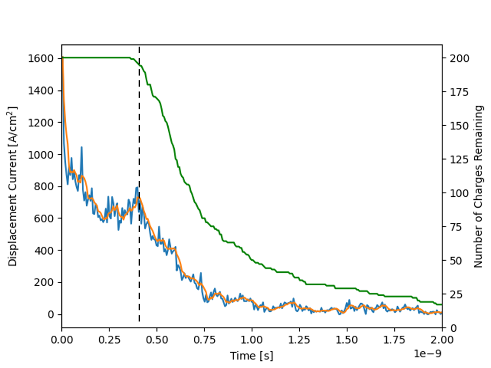
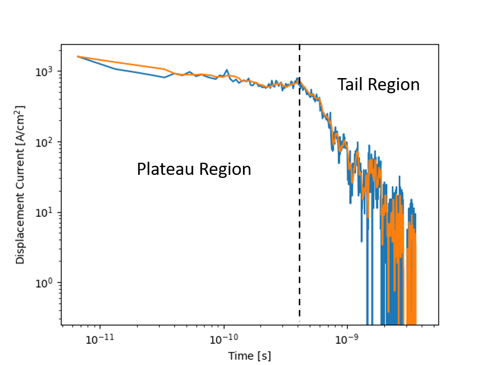
In the first image, you will notice that the current rapidly drops initially, this is what is referred to as hot carrier decay. As we randomly assigned charges to sites some of them would have ended up on high energy sites. It is easy for carriers in high energy sites to move because the energy barriers will be low. As they move, they loose energy and decay into lower energy sites where the energetic barriers to moving forward become larger. It is neat to see how the kinetic Monte Carlo calculations are able to capture this behavior. I would recommend the interested reader to take a look at actual experiments to see how well Monte Carlo simulations can capture the charge transport behavior. As an example consider the paper by T. Kreouzis et al. where they depict similar profiles for the photocurrent [4].
As the carriers continue to move through the material some of them become stuck in deep traps this is why there is a slope following the initial drop and is a result of dispersive transport where the signal becomes attenuated. The region where the current density begins to plateau is indicated to the left of the dotted line. Once the carriers start reaching the far electrode and are removed the current density drops again and is what causes the second slope seen in the tail region. The green line shown in linear plot clearly depicts where this transition occurs as it measures how many carriers remain in the active layer.
References
- J. Nelson, J. J. Kwiatkowski, J. Kirkpatrick, and J. M. Frost, “Modeling charge transport in organic photovoltaic materials,” Acc. Chem. Res., vol. 42, no. 11, pp. 1768–1778, 2009.
- A. Masse, Multiscale modeling of charge transport in organic devices : from molecule to device Multiscale modeling of charge transport in organic devices : from molecule to device. 2017.
- S. T. Hoffmann et al., “How do disorder, reorganization, and localization influence the hole mobility in conjugated copolymers?,” J. Am. Chem. Soc., vol. 135, no. 5, pp. 1772–1782, 2013.
- T. Kreouzis et al., “Temperature and field dependence of hole mobility in poly(9,9-dioctylfluorene),” Phys. Rev. B, vol. 73, no. 23, pp. 1–15, 2006.